Pressure Driven Nozzle Flow with Shock – rhoCentralFoam

In this post I will go over the set up and solution of a pressure driven nozzle flow with a shock located in the diverging section. This refers to the type of flow problem described by region b in my page covering stationary normal shock-waves.

Here is a summary of the contents of this post:

1. Nozzle Design
2. Mesh Generation
3. Boundary and Initial Conditions
4. Constants and Schemes
5. Running the Simulation/Results
6. Conclusion

The OpenFOAM file that is ready to download and run can be downloaded from here:

Nozzle with Shock Tutorial File Download

Simulation summary:

Nozzle Design Calculation

We want to simulate the flow in a converging-diverging nozzle, with a shock at a specified location in the diverging section. Based on the nozzle geometry we create we must calculate the required back pressure. This boundary condition will generate the shock in our nozzle.

Here is the nozzle geometry we will work with:

• Known nozzle height at through ()
• Known nozzle height at the outlet (, the outlet height is twice the throat height)
• Shock located when flow reaches M=1.88 (corresponding to A/A*=1.53)
• Stagnation Properties, Po=3 Bar, To=298K
• Fluid is air (γ=1.4)

To know how to set the back pressure, we must calculate the flow through the nozzle. This can be easily calculated by hand, using tables, or by using the Matlab app available from curiosityFluids.

The shock is to occur when the Mach number is 1.88. Therefore, we can calculate the preshock and post shock properties easily.

After the shock, the (now) subsonic flow is expanded out of the diverging section of the nozzle. We need to calculate the Mach number and pressure at the exit.

Recall that

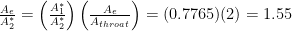
therefore

,

and

This is the approximate pressure at the outlet! This will be used for our downstream boundary condition!

Mesh Generation

To build the mesh we will use the native openFoam meshing utility blockMesh. For a detailed overview of the blockMesh utility it is best to start at with the OpenFoam user guide. Block mesh uses definitions of vertices, blocks, edges, and faces to define the mesh.

Vertices

Vertices define the shape of the boundary. I find it helpful to number the vertices in the file, and draw a diagram:

vertices
(
 (-0.6 0 -0.005) //0
 (-0.2121321 0 -0.005) //1
(0 0 -0.005) //2
 (2 0 -0.005) //3
(-0.6 0.45 -0.005) //4
 (-0.3 0.45 -0.005) //5
(0 0.15 -0.005) //6
 (2 0.3 -0.005) //7
(-0.6 0 0.005) //8
 (-0.2121321 0 0.005) //9
(0 0 0.005) //10
 (2 0 0.005) //11
(-0.6 0.45 0.005) //12
 (-0.3 0.45 0.005) //13
 (0 0.15 0.005) //14
 (2 0.3 0.005) //15 
 (-0.2121321 0.237867965 -0.005) //16
 (-0.2121321 0.237867965 0.005) //17
(-0.6 0.237867965 -0.005) //18
 (-0.6 0.237867965 0.005) //19
 (-4 0 -0.005) //20
 (-4 0.237867965 -0.005) //21
 (-4 0.45 -0.005) //22
 (-4 3.85 -0.005) //23
 (-0.6 3.85 -0.005) //24
 (-0.3 3.85 -0.005) //25
(-4 0 0.005) //26
 (-4 0.237867965 0.005) //27
 (-4 0.45 0.005) //28
 (-4 3.85 0.005) //29
 (-0.6 3.85 0.005) //30
 (-0.3 3.85 0.005) //31
);

Blocks

The blocks are used to define the different regions within the mesh. The blocks are defined here in a way to allow mesh inflation into the reservoir where the interesting flow is not occurring.

The blocks are defined below. The blocks with “simpleGrading” defined are the blocks that have an inflation applied to them.

blocks
(
 hex (9 8 19 17 1 0 18 16) (20 20 1) simpleGrading (1 1 1)
 hex (17 19 12 13 16 18 4 5) (20 20 1) simpleGrading (1 1 1)
 hex (10 9 17 14 2 1 16 6) (20 20 1) simpleGrading (1 1 1)
 hex (11 10 14 15 3 2 6 7) (150 20 1) simpleGrading (1 1 1)
 hex (12 28 29 30 4 22 23 24) (40 40 1) simpleGrading (10 10 1)
 hex (8 26 27 19 0 20 21 18) (40 20 1) simpleGrading (10 1 1)
 hex (19 27 28 12 18 21 22 4) (40 20 1) simpleGrading (10 1 1)
 hex (13 12 30 31 5 4 24 25) (20 40 1) simpleGrading (1 10 1)
);

Edges

We need to use an edge definition here in order to make a smooth subsonic inlet into the nozzle.

Below is the edge definition from the blockMeshDict:

edges
(
 arc 5 16 (-0.295442325 0.397905546 -0.005)
 arc 16 6 (-0.052094453 0.154557674 -0.005)
 arc 13 17 (-0.295442325 0.397905546 0.005)
 arc 17 14 (-0.052094453 0.154557674 0.005)
);

Boundaries

The face definition is very important as it defines the locations of all the pertinent boundaries, names them, and sets their boundary type. The faces are shown in the figure below. Notice that there is no definition for the front and back faces. This is because if you leave them undefined blockMesh adds them to a group of faces called defaultFaces which we can then later define as empty.

The boundary definitions from the blockMeshDict are shown below:

boundary
(
 inlet1
 {
 type patch;
 faces
 (
 (20 26 27 21)
 (21 27 28 22)
 (22 28 29 23)
 );
 }
 top
 {
 type wall;
 faces
 (
 (23 29 30 24)
 (24 30 31 25)
 );
 }

outlet
 {
 type patch;
 faces
 (
 (11 3 7 15)
 );
 }
 bottom
 {
 type symmetryPlane;
 faces
 (
 (8 0 1 9)
 (9 1 2 10)
 (10 2 3 11)
 (26 20 0 8)
 );
 }
 nozzle
 {
 type wall;
 faces
 (
 (5 13 17 16)
 (16 17 14 6)
 (6 14 15 7)
 (13 5 25 31)
 );
 }
);

Build Mesh

To build the mesh simply type blockMesh into the command terminal from inside you case file. To ensure the mesh built properly, then run checkMesh .

Boundary and Initial Conditions

Once the mesh is built, it is time to set up the case. The boundary and initial conditions are defined in the “0” folder. The solver for this case is rhoCentralFoam which requires P, T, U definitions in the 0 folder. A summary of the boundary conditions and the mesh resulting from the previous section is shown in the next picture:

Initial Conditions

Here I/we have initialized the internalField the simulation with a small x-velocity (7 m/s), pressure equal to the stagnation pressure, and temperature equal to 298 K.

Boundary Conditions

There are some key aspects of this setup that are essential to setting up this problem. The first is the totalPressure  definition for the inlet pressure. This boundary condition maintains the inlet at a constant stagnation pressure. This allows this boundary to behave like an infinite reservoir. To complement this boundary condition we use the zeroGradient boundary conditions for velocity. By setting velocity to zeroGradient, we are allowing flow to be induced by the nozzle. If you set a fixedValue for the velocity, you would be constraining the amount of mass flow into the system, and therefore would require some extra set-up calculations. Additionally, you would be making the use of the totalPressure boundary condition obsolete. For the temperature we set a fixed value at 298 K. This maintains the flow induced from the nozzle at a constant temperature.

For the outlet we want to ensure that the correct back pressure is maintained. This will make sure that we have a shock forming in the nozzle. Temperature and velocity are set to zeroGradient and therefore will be determined by the nozzle flow.

The symmetry plane is set by setting p, T, and U to be type symmetry. 

The nozzle boundary should be set to type slip for velocity. This ensures that flow tangency is maintained for velocity (but we are not enforcing the no-slip condition as this is an inviscid simulation). For pressure, and temperature zeroGradient should be used. This makes the wall adiabatic (i.e. no heat flux) and makes the pressure calculated by the flow.

Below is a summary of p, T, and U files that should be in your “0” folder:

p

dimensions [1 -1 -2 0 0 0 0];

internalField uniform 3000000;

boundaryField
{
 inlet1
 {
 type totalPressure;
 p0 uniform 3000000;
 gamma 1.4;
 value $internalField;
 }

outlet
 {
 type fixedValue;
 value uniform 2067400;
 }

bottom
 {
 type symmetryPlane;
 }
 top
 {
 type zeroGradient;
 }

nozzle
 {
 type zeroGradient;
 }

defaultFaces
 {
 type empty;
 }
}

T

dimensions [0 0 0 1 0 0 0];

internalField uniform 298;

boundaryField
{
 inlet1
 {
 type fixedValue;
 value uniform 298;
 }

outlet
 {
 type zeroGradient;
 }
 top
 {
 type slip;
 }
 bottom
 {
 type symmetryPlane;
 }

nozzle
 {
 type zeroGradient;
 }
defaultFaces
{
 type empty;
 }
}

U

dimensions [0 1 -1 0 0 0 0];

internalField uniform (7 0 0);

boundaryField
{
 inlet1
 {
 type zeroGradient;
 }

outlet
 {
 type zeroGradient;
 }

bottom
 {
 type symmetryPlane;
 }
 top
 {
 type slip;
 }

nozzle
 {
 type slip;
 }

defaultFaces
 {
 type empty;
 }
}

Constants and Schemes

thermophysicalProperties

As the name states, in the thermophysicalProperties file we will specify the thermophysicalProperties of the gas.

thermoType
{
 type hePsiThermo;
 mixture pureMixture;
 transport const;
 thermo hConst;
 equationOfState perfectGas;
 specie specie;
 energy sensibleInternalEnergy;
}

mixture
{
 specie
 {
 nMoles 1;
 molWeight 29;
 }
 thermodynamics
 {
 Cp 1005;
 Hf 0;
 }
 transport
 {
 mu 0;
 Pr 1;
 }
}

In the file shown above, we have defined the simulation fluid is an ideal gas with Cp=1005, and a molar mass of approximately 29. This gives the approximate properties of air. We set the viscosity mu=0 because the simulation is inviscid.

fvSchemes

Usually, the fvSchemes from the rhoCentralFoam tutorials are good enough. However, I always change the flux limiter from vanLeer to vanAlbada. This is because, in my experience, it works much better at removing spurious oscillations from the flow-field. There are other options that I change occasionally, but for this wedge simulation that is the only parameter I have altered. The limiter option is found in the interpolationSchemes section:

interpolationSchemes
{
 default linear;
 reconstruct(rho) vanAlbada;
 reconstruct(U) vanAlbadaV;
 reconstruct(T) vanAlbada;
}

Running the Simulation/Results

Running rhoCentralFoam

Once the case is set up, it is time to run the simulation. To run the simulation you simply type rhoCentralFoam into the terminal from inside the case file.

Establishing convergence in time

In order to reach the final answer, the simulation must be run for a long time. Why? This is a limitation due to how we have chosen to approach this problem. Here we are using rhoCentralFoam which is an unsteady solver. The problem we are examining here is in fact a steady problem. So in order to achieve the answer we have to run from our arbitrary (but not insignificant) initial conditions, until the simulation stops changing in time. In steady-state solvers, the terms of the governing equations are manually fixed to zero. The remaining equation is then solved iteratively until convergence. Here, we solve forward in time until the  terms approach zero eventually.

Recall that because of our boundary conditions, the inlet velocity is an output of the simulation. Here, I have chosen to use this as the variable for which I will test convergence in time. The following graph shows the inlet velocity as a function of time at a node along the inlet face.

As you can see from the picture, the inlet velocity fluctuates significantly at the beginning of the simulation. However by the end of the simulation time it has converged on a constant value.

This is a downside of the current approach. However, there are ways to speed up convergence such as the application of a relaxation factor in time, or the use of a non-reflective boundary condition. I will not go into detail regarding those here.

Results and Analysis

Below are contour plots showing the solution results.

Are the results what we expected?

At first glance it appears that the simulation is good. As designed, we have a stationary normal shock standing in the diverging section of the nozzle. To analyze this further I have taken the Mach number along the centerline of the diverging section and calculated the corresponding A/A*.

We designed the nozzle to produce a shock at a specific location (A/A*) in the nozzle. From the figure above, we can see that the A/A* where the shock occurs is slightly higher than the design point. Similarly the  A/A* at the nozzle exit is higher than the design point. There are several reasons that this could be. For one, this simulation is two-dimensional and the flow properties are not constant in the y-direction. If we were to be rigorously comparing to the 1D calculation, we would probably need to either (a) average the Mach number at each length-wise station or (b) extend the nozzle to be significantly longer. Another possibility is (again since the simulation is 2D) that the Prandtl-Meyer waves emanating from the throat upset the accuracy of the simulation. These waves are visible in the figure above. These waves occur because of the finite change in angle between the throat and the straight diverging section. This could be avoid in future simulations by: (a) modelling the transition from throat to diverging section smoothly, or by (b) extending the length of the diverging section

What are some of the observed limitations? Improvements?

The biggest and most obvious limitation of this simulation (in my opinion) is the finite angle change that was used to create the geometry. This produced a Prandtl-Meyer expansion fan that hurt the quality of the simulation. If we were to improve this simulation, I would extend the diverging section to be much longer to reduce this finite angle change.

Another limitation of this simulation is that it is inviscid. While it is interesting and useful to compare to the analytical 1D solutions, in real life viscosity has a very real and important affect on the flow result.

Some improvements could be made to the simulation numerically as well. First of all, the grid used in the simulation was made coarse so that the simulation time would be small. A finer grid will produce a higher resolution image of the shock wave and an overall better result. Similarly, the size of the timestep could be decrease to lower the simulation CFL number. Some spurious oscillations can be seen in the post-shock section of the nozzle. These will be reduced by lowering the CFL.

Conclusions

In this post, we designed and simulated a converging diverging nozzle connected to a reservoir using the OpenFOAM solver rhoCentralFoam. The simulation produced the expected results. However, the finite angle change used to model the nozzle geometry produced expansion waves which hurt the quality of the simulation.

Please provide comments and suggestions on improvements!

curiosityFluids