Solving the cavity flow problem using the streamfunction-vorticity formulation

In this post I am going to write a (hopefully) simple code in matlab to solve the cavity flow problem using the vorticity stream function formulation. I will the compare the result to the result calculated by the OpenFOAM solver, icoFoam.  Writing your own solvers is fun, rewarding, and is a practice that really cements some of the fundamental knowledge of CFD.

Contents

1. Introduction to the Cavity Flow Problem
2. Governing Equations
3. Finite Differences and Solver Algorithm
   • Understanding and setting the boundary conditions
   • Semi-discretization of the governing equations
   • Solving the vorticity equation in time
   • Solving for the vorticity at the boundaries
   • Solving for the stream function
   • Putting it all together
4. Results/Comparison to icoFoam
   • Re=10
   • Re=100
5. Conclusion and some References

Introduction to the Cavity Flow Problem

The cavity flow problem is described in the following figure. Basically, there is a constant velocity across the top of the cavity which creates a circulating flow inside. To simulate this there is a constant velocity boundary condition applied to the lid, while the other three walls obey the no slip condition. Different Reynolds numbers give different results, so in this post I’ll simulate Re=10, and Re=800. At high Reynolds numbers we expect to see a more interesting result with secondary circulation zones forming in the corners of the cavity.

Governing Equations

To start let’s remember that in 2D incompressible flow the Navier-Stokes equations can be rewritten to form the following two equations:

 (1)

   (2)

The two equations above are easily derived and I will probably make a short blog post covering it. For now you can take my word for it… these solve a major complication of the Navier-Stokes equations and that is the pressure-velocity coupling! By making a change of variables from u, v, and p, to and this is now in a simpler form to solve numerically.

Finite differences and solver algorithm

Understanding the boundary conditions

Quickly I need to explain the boundary conditions for this problem. They seem simple enough, velocity top and no velocity on the left, bottom and right sides. But remember there is no velocity in our equations! We have stream-function and vorticity. So how do we set our boundary conditions?! Well, the trick is to recognize that the outside can be considered a closed streamline. Meaning that all around the edge it will have a constant value of stream function. What should the value be? It actually doesn’t matter. But most commonly you’ll see this be set at . This helps simplify some parts of the problem as you’ll see later. And what about vorticity? There is actually no boundary condition for vorticity in fact. It is an output of the simulation. At each iteration of the solver we must calculate the value of the vorticity at the wall either from the stream function or by using the same method for calculating the rest of the vorticity points. I’ll explain how we do this once we get a little further on.

Semi-discretization of the governing equations

Now, we are going to use finite differences to discretize the equations and create a system of equations that can be solved.  Finite differences are used to approximate the derivatives at each point using the surrounding points that are a finite distance away. This is shown in the next figure. By doing this we create one equation for each node inside the cavity. When all of these equations are put together they form a system of equations that can be solved.

In the stream-function vorticity formulation there are only first and second derivatives in x and y, and a first derivative in time. For these we are going to use the finite difference equations summarized below (Eqs 3-6) which are all 2nd order.

First partial derivatives: (3)    (4)  

Second partial derivatives (5)  (6) 

The first step is to insert equations 3-6 into equations 1 and 2. We now have a set of vorticity stream function equations based on finite differences. For simplicity I will solve this problem on a perfectly square grid where . This allows the equations and the coding to be much simpler. We end up with:

(7) (rearranged for and simplified)

(8)

Next the process can go several ways. We can solve Equation 1 and 2 simultaneously or sequentially, and we could solve Equation 1 first or Equation 2 first. As well we could modify the equations based on some information we already know to be true. For instance, we know ahead of that this problem is a “steady state problem” which means that it doesn’t vary in time. Yet, equation 2 has  a time derivative in it. In one approach, we could get rid of this term from the equation which we know to be zero and write a steady state solver. Alternatively (and the way I chose to do it here) is we use that time derivative to solve the equation in time and as the time gets large (as ) the simulation should stop changing and the time derivative would go to zero. Here we are going to solve the equations sequentially starting with the vorticity equation using the time derivative (Equation 2) followed by Equation 1.

Solving the vorticity equation in time

So to use this  approach we are going to use the most simple time discretization – the explicit Euler scheme (1st order). The easiest way to think about this is we can rearrange Equation 2 to give an equation of the form:

(9)

where f(x) is the function formed by our finite difference equations. We then know from the first order Taylor series that we can say:

(10)

where: 

Here k means the time step index. Meaning k is the current time step and k+1 is the next time step. is the chosen time step size. This must be chosen based on stability, or a desired time accuracy. Using the equation above we can predict the vorticity throughout the field at the next timestep. This is really the key to the solver we are writing.

Solving for the vorticity at the boundaries

In the last step I showed how the vorticity can be predicted in time using the explicit Euler formulation. But this is not all that needs to be done to define the vorticity. In the middle points all of the central differences are valid because all of the points have neighbors in all directions. However, at the boundaries things get a little interesting. They don’t have a full set of neighbors! For example on the left there are no nodes for which to use in the central difference equations. There are a couple different ways to do this. The most obvious way is to use one-sided finite differences to formulate the equations at these nodes. However there is an easier way that comes from a simple observation of the Taylor series.

Using the top wall as an example, from Equation 1 we know that:

(11)

This is because the stream function is constant along the top and therefore . From the Taylor series we know that

(12)

There are several properties in the above expansion that we know. For instance, , and also that . By subbing these in and rearranging for vorticity we get:

(13)

We also know that we set so the actual equation for the top boundary becomes:

(14a)  (top)

Similarly equation for the other boundaries are:

(14b)  (bottom)

(14c) (left)

(14d) (right)

Solving for the streamfunction

After predicting the vorticity at the next time step, we can solve Equation 1 for the corresponding stream function. To solve Equation 1, the way that I have chosen to do it is to rearrange the finite difference equation for the stream-function psi at indices i,j:

(15)

Then it is a matter of using a simple loop structure (probably a for loop) to loop through all the nodes and calculate the predicted psi. Since we are running until we reach steady state, after each time step we should check the value of the time derivative and when it reaches an acceptably small value we will call the simulation converged.

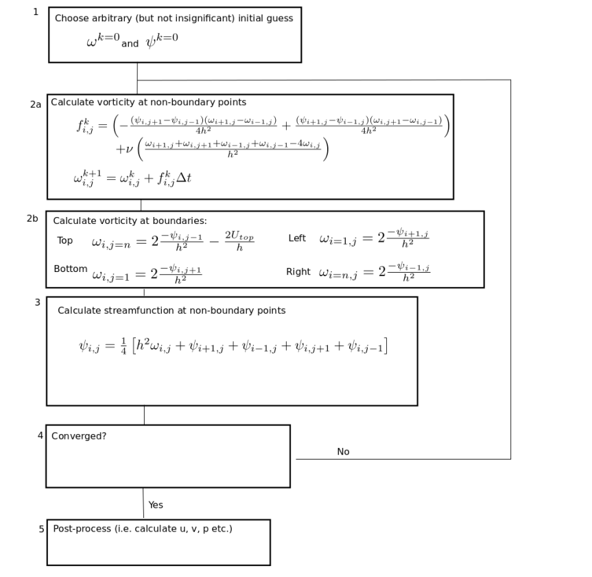
Putting it all together

So to summarize the steps for the solver are:

1. Choose an arbitrary starting point (ie assuming a streamfunction and vorticity at all points)
2. a) Loop through all interior nodes and calculate the time derivative , and use explicit Euler to guess the vorticity at each point at the next time-step (k+1)
   b) At boundary nodes, calculate the vorticity at the boundaries using the simple Taylor series approximation
3. Loop through all interior nodes and solve Equation 1 to predict the stream-function. Keep the stream-function at all boundaries the same ()
4. Check for convergence (based on some user defined criteria)
5. If converged the simulation is done, you can now post-process and calculate things such as velocity and pressure. If not converged go back to step 2 and continue forward solving in time.

Below is a schematic summary of the solver algorithm I just described:

Results

To examine the results of my solver I am going to simulate two Reynolds numbers 10, and 800 using both my own solver, and the OpenFoam solver on a comparable grid size. I am assuming the OpenFoam solver to be the superior being since it is written by folks much smarter than I. The OpenFOAM solver that I am using is the solver icoFoam. And coincidentally the OpenFOAM download comes with the cavity problem already set up and all I had to do was hit run! … (After changing the Reynolds number and grid size of course)

Re = 10

Because of the low Reynolds number I expected both solvers to perform similarly. I compared the output velocity, streamfunction, and vorticity fields. Both of the simulations were done on a 60×60 grid. Take a look:

At this Reynolds number it seems like my solver did a pretty darn good job! The stream function, vorticity, and velocity plots match quite closely. And they look kinda pretty too! I plotted the OpenFOAM output in Matlab so that the images would be plotted the same. Comparing matlab to Paraview just didnt do it for me. Maybe I’ll do a blog about but putting openfoam into Matlab… at a later date.

Re = 800

Re 800 is supposed to be a much more challenging case. Why? Well for one… the Reynolds number is higher. This means that shear layers are thinner compared to the problem length scale and therefore require more resolution. Additionally, we (or I anyway) know that at these Reynolds numbers reversed flow and separation bubbles are produced in the corners.

For this one each simulation (both icoFoam and the matlab solver I wrote) are solved on a 100×100 grid. The higher resolution is necessary because of the more complex flow. So… lets see how it went!

On thing we notice right away is how much prettier Re 800 is! But again it looks like the solvers match up pretty closely! The vorticity plots are on a log scale. This is a great example of the flow described by Batchelor about high Reynolds number flow with closed streamlines. We have vorticity being convected around the outside of a mostly constant vorticity core.

Conclusion and some References

If you read this far… thanks for paying attention! This was my first post and first time writing a solver with (maybe) some people watching/reading. If anything is unclear or incorrect (I do make lots of mistakes) comment or something. Here is a link to the matlab code I wrote! Feel free to use it… but if you publish anywhere please reference it: streamvortRe10

Some useful references and alternative sources if you are very interested in this method are:

Website pages:

[1] https://www.iist.ac.in/sites/default/files/people/psi-omega.pdf

[2] http://nptel.ac.in/courses/112104030/pdf/lecture24.pdf

[3] http://www.cfm.brown.edu/people/gk/chap11/node1.html

[4] http://www.hindawi.com/journals/isrn/2012/871538/

Books

[5] J. C. Tannehill, D. A. Anderson, R. H. Pletcher”Incompressible Navier-Stokes Equations”, Computational Fluid Mechanics and Heat Transfer, 2nd Edition, Taylor and Francis, 1997, pp. 649-659

[6] K. H. Huebner, E. A. Thornton, T. G. Byrom ,”Fluid Mechanics Problems” The Finite Element Method for Engineers, 2nd Edition, John Wiley and Sons, 1995

OpenFOAM

[7] OpenCFD, “OpenFOAM- The Open Source Computational Fluid Dynamics (CFD) Toolbox”, http://www.openfoam.com